Identify the Optimal Number of Clusters Based on Maximum Fusion Height

Identifies the number of clusters corresponding to the largest increase in fusion height in a hierarchical clustering dendrogram.

Usage

maxFusionLevel(cluster)

Arguments

cluster

An object of class hclust, typically obtained using stats::hclust().

Value

A list containing:

n.clust

Integer vector indicating the number of clusters corresponding to the maximum increase in fusion height. Multiple values may be returned in the case of ties.

results

A data frame containing:

• h: fusion heights.

• n.clust: number of clusters before each fusion.

• diff: differences between consecutive fusion heights.

Details

The function calculates the difference between consecutive fusion heights obtained from a hierarchical clustering analysis.

The optimal number of clusters is identified as the number of groups immediately before the largest increase in fusion height.

A large increase suggests that relatively dissimilar clusters are being merged, potentially indicating a meaningful partition of the dataset.

This is a heuristic criterion and does not guarantee the identification of the ecologically or statistically optimal number of clusters. Results may depend on the distance measure and linkage method used.

See also

hclust, cutree

#' @references Borcard, D., Gillet, F., & Legendre, P. (2018). Numerical Ecology with R (2nd ed.). Springer, Cham. https://doi.org/10.1007/978-3-319-71404-2

Examples

# Hierarchical clustering using the USArrests dataset
data(USArrests)

d <- dist(scale(USArrests))
hc <- hclust(d, method = "ward.D2")

# Identify the number of clusters
res <- maxFusionLevel(hc)

# Suggested number of clusters
res$n.clust
#> [1] 2

# Fusion heights and their differences
res$results
#>             h n.clust        diff
#> 1   0.2058539      50          NA
#> 2   0.3502188      49 0.144364899
#> 3   0.4287712      48 0.078552416
#> 4   0.4940832      47 0.065312015
#> 5   0.5353893      46 0.041306068
#> 6   0.5535286      45 0.018139387
#> 7   0.5935343      44 0.040005700
#> 8   0.6559259      43 0.062391556
#> 9   0.7038309      42 0.047905009
#> 10  0.7108812      41 0.007050268
#> 11  0.7389936      40 0.028112413
#> 12  0.7722224      39 0.033228861
#> 13  0.7781298      38 0.005907377
#> 14  0.7865674      37 0.008437523
#> 15  0.7977642      36 0.011196804
#> 16  0.8076434      35 0.009879204
#> 17  0.8472042      34 0.039560844
#> 18  0.9427614      33 0.095557211
#> 19  0.9513719      32 0.008610445
#> 20  0.9824857      31 0.031113824
#> 21  1.0122252      30 0.029739526
#> 22  1.0598104      29 0.047585190
#> 23  1.0709720      28 0.011161575
#> 24  1.0756115      27 0.004639495
#> 25  1.0910920      26 0.015480576
#> 26  1.1606271      25 0.069535066
#> 27  1.1968261      24 0.036198967
#> 28  1.2074603      23 0.010634257
#> 29  1.2601290      22 0.052668642
#> 30  1.2990516      21 0.038922610
#> 31  1.3169658      20 0.017914169
#> 32  1.3449118      19 0.027946047
#> 33  1.3901014      18 0.045189630
#> 34  1.5396377      17 0.149536250
#> 35  1.6907596      16 0.151121938
#> 36  1.7484165      15 0.057656842
#> 37  1.8118061      14 0.063389664
#> 38  1.9360777      13 0.124271589
#> 39  2.2033391      12 0.267261385
#> 40  2.2421782      11 0.038839123
#> 41  2.7145543      10 0.472376097
#> 42  2.9932892       9 0.278734904
#> 43  3.0250236       8 0.031734392
#> 44  3.2107135       7 0.185689846
#> 45  3.4960481       6 0.285334652
#> 46  3.7341155       5 0.238067364
#> 47  6.4618664       4 2.727750963
#> 48  7.1881893       3 0.726322905
#> 49 13.5162424       2 6.328053004

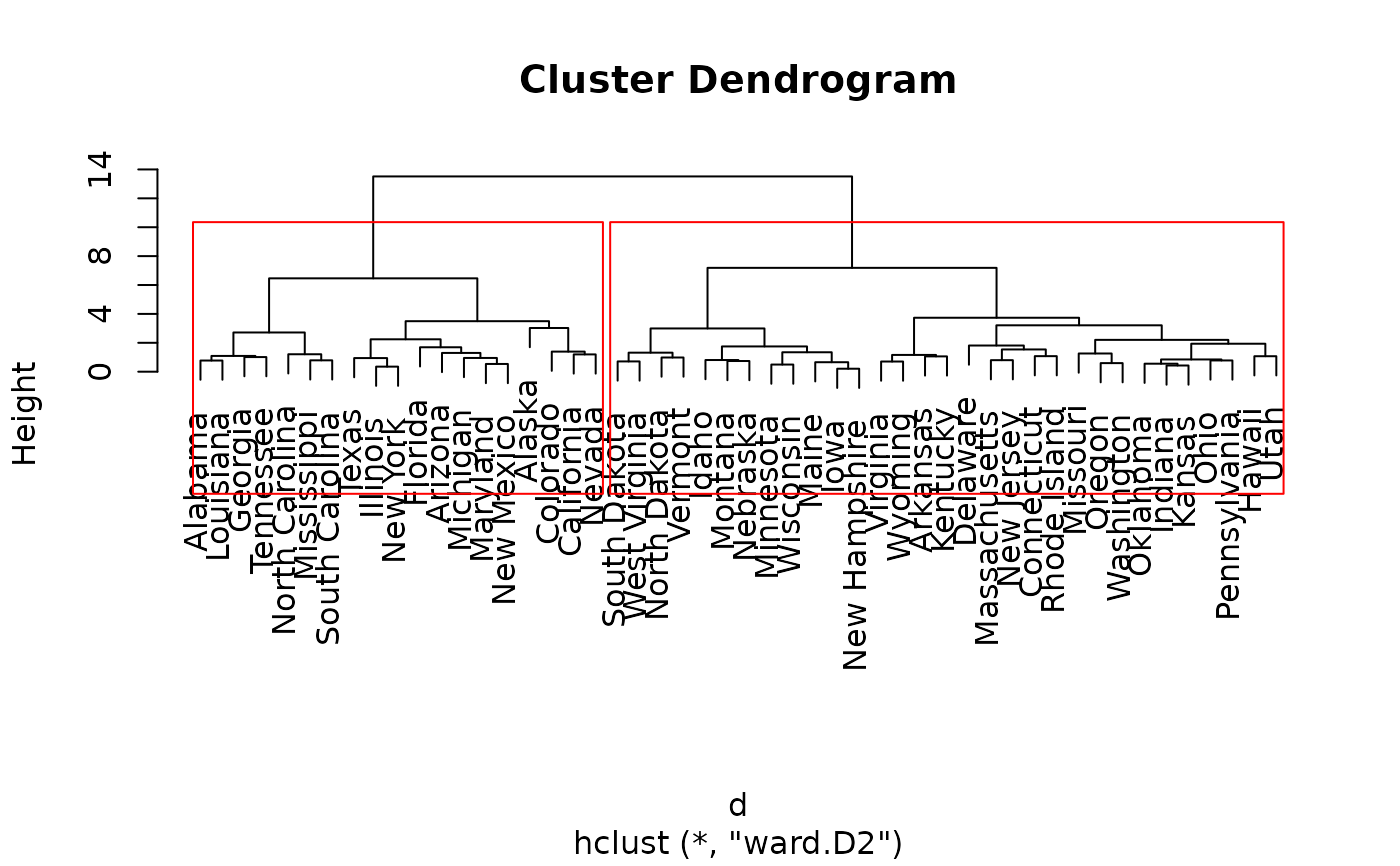
# Plot the dendrogram with the suggested partition
plot(hc)
rect.hclust(hc, k = res$n.clust[1], border = "red")