Vegetation classification: a phytosociological approach

Marco Pittarello

This vignette illustrates classification using modified TWINSPAN and selection of the number of groups using OptimClass. The resulting groups are then described using Indicator Species Analysis (ISA), the phi coefficient, tb-PCA, and a synoptic table.

The example uses only iPastoralist::data. For this example, survey values are assumed to represent percentage cover, although the demonstration dataset was originally organised as frequencies of occurrence. This assumption illustrates the workflow; it is not a methodological conversion from FO to cover. Real applications require observed cover values and careful consideration of the measurement scale.

1. Required packages and functions

TWINSPAN requires a version of ecan that exports twinspan().

library(iPastoralist)
library(vegan)
library(indicspecies)
library(permute)

2. Preparing cover data

data_example <- as.data.frame(iPastoralist::data)
data_example <- data_example[, c(2, 7:30)]

cover <- iPastoralist::vegetation_abundance(
  database = data_example,
  species.cover.coefficient = 4,
  method = "SC_fo_occ"
)

# Rows = surveys; columns = species.
veg <- t(cover)

dim(veg)
#> [1]  24 152
knitr::kable(veg[seq_len(min(6L, nrow(veg))), seq_len(min(6L, ncol(veg)))])

	Achmacr	Achmill	Achmosc	Acialpi	Acolama	Adealli
R1	0	0	0	0	0.3	0.0
R2	0	0	0	0	0.0	0.3
R3	0	0	0	0	0.0	0.0
R4	0	0	0	0	0.0	0.0
R5	0	0	0	0	0.0	0.0
R6	0	0	0	0	0.0	0.0

3. Modified TWINSPAN and OptimClass

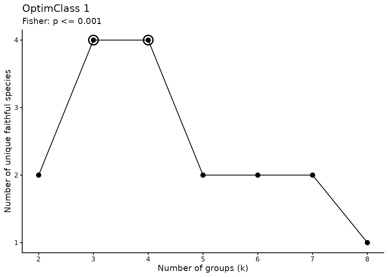
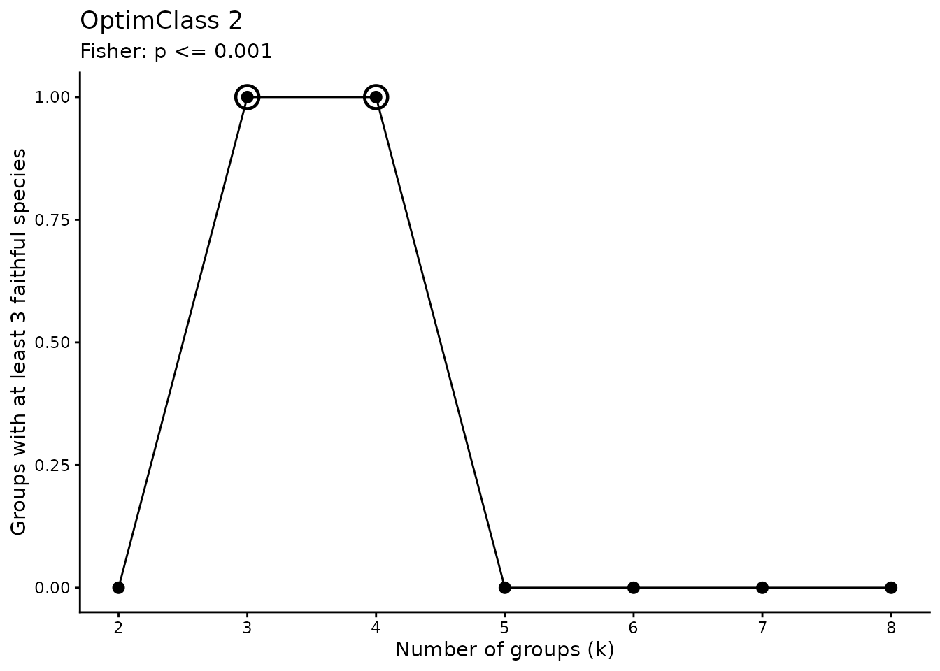
TWINSPAN uses pseudospecies cut levels to represent abundances. Here, the cover thresholds are 0, 2, 5, 10, and 20. Modified TWINSPAN prioritises splitting the most heterogeneous group. OptimClass compares partitions based on faithful species: OptimClass 1 considers the total number of faithful species, whereas OptimClass 2 considers the number of groups containing a sufficient number of faithful species (Tichý et al., 2010).

The significance threshold and minimum number of faithful species are analysis parameters that should be reported and assessed for your dataset. The range of group numbers examined here is also limited by the small size of the demonstration dataset.

min_size <- 2L
k_values <- 2:8
cut_levels <- c(0, 2, 5, 10, 20)
p_threshold <- 1e-3
min_faithful <- 3L
select_by <- "optimclass2" # alternative: "optimclass1"

In the ecan backend, min_size controls which groups can be split further; on its own, it does not guarantee that every final group contains at least that many surveys. Always check final group sizes after classification.

twinspan_res <- twinspan_optimclass_ecan(
  veg = veg,
  cut_levels = cut_levels,
  min_size = min_size,
  k_values = k_values,
  p_threshold = p_threshold,
  min_faithful = min_faithful,
  version = "fast",
  select_by = select_by,
  show_plots = TRUE
)

#> 
#> --- TWINSPAN + OPTIMCLASS ---
#> Version: fast 
#> OptimClass 1, optimal k values: 3, 4 
#> OptimClass 2, optimal k values: 3, 4 
#> Selected partition:3groups (optimclass2)
#> Unique faithful species: 4

knitr::kable(twinspan_res$results)

k	optimclass1	optimclass2	prop_good_clusters	min_group_size	best_optim1	best_optim2
2	2	0	0.0000000	4	FALSE	FALSE
3	4	1	0.3333333	4	TRUE	TRUE
4	4	1	0.2500000	3	TRUE	TRUE
5	2	0	0.0000000	3	FALSE	FALSE
6	2	0	0.0000000	3	FALSE	FALSE
7	2	0	0.0000000	1	FALSE	FALSE
8	1	0	0.0000000	1	FALSE	FALSE

twinspan_res$best_k
#> $optimclass1
#> [1] 3 4
#> 
#> $optimclass2
#> [1] 3 4
twinspan_res$selected_k
#> [1] 3

Also examine the faithful species of the selected solution. Species used by OptimClass to select a partition may differ from those subsequently selected using IndVal or phi: the criteria and thresholds are not interchangeable.

twinspan_res$faithful_by_group
#> $G1
#> character(0)
#> 
#> $G2
#> [1] "Cerarve" "Myoalpe" "Phybeto" "Potgran"
#> 
#> $G3
#> character(0)
head(twinspan_res$faithful_species)
#>   k group species      p_value
#> 3 3    G2 Cerarve 1.458249e-04
#> 4 3    G2 Myoalpe 7.189271e-05
#> 5 3    G2 Phybeto 3.701710e-04
#> 6 3    G2 Potgran 5.103872e-04

4. Selecting the partition and aligning groups

The default solution is the one returned by OptimClass. If no single valid selected_k is returned, examine results and best_k and choose a solution explicitly. For example, a maximum OptimClass 2 score of zero does not demonstrate that the groups meet the desired faithful-species requirement.

n.cluster <- twinspan_res$selected_k
groups_raw <- as.data.frame(twinspan_res$classification)

To assess an alternative solution, run the following chunk instead of the previous one. It is excluded from normal rendering with eval = FALSE to avoid automatically overwriting the OptimClass selection. After running it manually, rerun all subsequent chunks, starting with group alignment.

k_custom <- 4L

twin_ecan <- ecan::twinspan(
  x = veg,
  modified = TRUE,
  n_clusters = k_custom,
  cut_levels = cut_levels,
  min_size = min_size,
  max_depth = 6,
  polish = "hill",
  species = FALSE
)

groups_raw <- as.data.frame(twin_ecan$classification[, c("stand", "group")])
n.cluster <- length(unique(groups_raw$group))
if (n.cluster != k_custom) {
  stop("TWINSPAN did not reach the requested number of groups.")
}

# Convert using the ecan S3 method, without calling internal functions.
hc_ecan <- stats::as.hclust(twin_ecan)
plot(hc_ecan, hang = -1, sub = "", main = "TWINSPAN - alternative solution")

Retain the partition in classification: do not derive a new classification by applying cutree() to the displayed dendrogram. Recode group labels as 1, 2, etc., and store them as a factor with the same level order for ISA, phi, PCA, and the synoptic table. This ensures that the version of synoptic_table() that adds a G prefix to frequency columns produces G1, G2, etc.

groups <- groups_raw[
  match(rownames(veg), as.character(groups_raw$stand)),
  c("stand", "group"),
  drop = FALSE
]
rownames(groups) <- NULL

# Retain the mapping to the original group labels.
original_group_levels <- levels(factor(groups$group))
group_key <- data.frame(
  original_group = original_group_levels,
  group = seq_along(original_group_levels)
)
groups$group <- factor(
  match(as.character(groups$group), original_group_levels),
  levels = seq_along(original_group_levels)
)

stopifnot(
  identical(rownames(veg), as.character(groups$stand)),
  !anyNA(groups$group),
  nlevels(droplevels(groups$group)) == n.cluster
)

knitr::kable(group_key)

original_group	group
G1	1
G2	2
G3	3

knitr::kable(groups)

stand	group
R1	2
R2	1
R3	1
R4	1
R5	2
R6	2
R7	2
R8	2
R9	2
R10	2
R11	2
R12	2
R13	3
R14	1
R15	2
R16	3
R17	1
R18	2
R19	1
R20	2
R21	2
R22	2
R23	3
R24	3

table(groups$group)
#> 
#>  1  2  3 
#>  6 14  4

5. Indicator Species Analysis

Calculate IndVal from cover data, using func = "IndVal.g" to account for unequal group sizes. Setting duleg = TRUE searches for species associated with individual groups, excluding combinations of groups.

The 9999 permutations are shared with the phi analysis. They are unrestricted in this example; a blocked design or repeated surveys require constraints consistent with the sampling design.

set.seed(123)
nperm <- 499L #to be fast here (better 9999)
indval <- indicspecies::multipatt(
  x = veg,
  cluster = groups$group,
  func = "IndVal.g",
  duleg = TRUE,
  permutations = nperm
)

summary(indval, alpha = 0.05, indvalcomp = TRUE)
#> 
#>  Multilevel pattern analysis
#>  ---------------------------
#> 
#>  Association function: IndVal.g
#>  Significance level (alpha): 0.05
#> 
#>  Total number of species: 152
#>  Selected number of species: 34 
#>  Number of species associated to 1 group: 34 
#>  Number of species associated to 2 groups: 0 
#> 
#>  List of species associated to each combination: 
#> 
#>  Group 1  #sps.  7 
#>              A      B  stat p.value   
#> Peuostr 0.9883 0.8333 0.908   0.005 **
#> Rumalpe 0.7240 1.0000 0.851   0.025 * 
#> Adealli 1.0000 0.6667 0.816   0.015 * 
#> Verlobe 0.9955 0.6667 0.815   0.015 * 
#> Luzalpi 0.9571 0.6667 0.799   0.040 * 
#> Descesp 0.9908 0.5000 0.704   0.025 * 
#> Taroffi 0.8750 0.5000 0.661   0.035 * 
#> 
#>  Group 2  #sps.  20 
#>              A      B  stat p.value   
#> Myoalpe 0.9923 0.9286 0.960   0.005 **
#> Chahirs 0.9859 0.9286 0.957   0.005 **
#> Camsche 0.9271 0.9286 0.928   0.015 * 
#> Ranmont 0.9209 0.9286 0.925   0.010 **
#> Fesnigr 0.8458 1.0000 0.920   0.005 **
#> Lotalpi 0.9293 0.8571 0.892   0.015 * 
#> Cerarve 1.0000 0.7857 0.886   0.015 * 
#> Geumont 0.9028 0.8571 0.880   0.010 **
#> Triprat 0.8862 0.8571 0.872   0.020 * 
#> Antalpi 0.8762 0.8571 0.867   0.005 **
#> Phybeto 0.8743 0.8571 0.866   0.050 * 
#> Potgran 1.0000 0.7143 0.845   0.020 * 
#> Silvulg 0.8854 0.7857 0.834   0.035 * 
#> Agrcapi 0.6929 1.0000 0.832   0.010 **
#> Galpusi 1.0000 0.6429 0.802   0.045 * 
#> Pulapii 1.0000 0.6429 0.802   0.035 * 
#> Phlrhae 0.6327 1.0000 0.795   0.015 * 
#> Cardefl 0.9680 0.5714 0.744   0.050 * 
#> Bislaev 1.0000 0.5000 0.707   0.045 * 
#> Leuvulg 1.0000 0.5000 0.707   0.020 * 
#> 
#>  Group 3  #sps.  7 
#>              A      B  stat p.value   
#> Rhoferr 0.8543 1.0000 0.924   0.005 **
#> Junnana 0.9965 0.7500 0.864   0.015 * 
#> Calvill 0.9209 0.7500 0.831   0.015 * 
#> Oxaacet 1.0000 0.5000 0.707   0.030 * 
#> Astmino 0.6632 0.7500 0.705   0.050 * 
#> Arnmont 0.9790 0.5000 0.700   0.025 * 
#> Gymdryo 0.9333 0.5000 0.683   0.035 * 
#> ---
#> Signif. codes:  0 '***' 0.001 '**' 0.01 '*' 0.05 '.' 0.1 ' ' 1

The A.g component describes indicator specificity, whereas B describes the frequency of the species within the group. The stat value returned by multipatt() is the square root of IndVal.

6. Phi coefficient

For phi, convert cover values to presence/absence. With func = "r.g", the association is adjusted for unequal group sizes. Occasional species with a cover value of 0.3 are therefore considered present.

veg_pa <- 1L * (veg > 0)

set.seed(123)
phi <- indicspecies::multipatt(
  x = veg_pa,
  cluster = groups$group,
  func = "r.g",
  duleg = TRUE,
  permutations = nperm
)

summary(phi, alpha = 0.05)
#> 
#>  Multilevel pattern analysis
#>  ---------------------------
#> 
#>  Association function: r.g
#>  Significance level (alpha): 0.05
#> 
#>  Total number of species: 152
#>  Selected number of species: 35 
#>  Number of species associated to 1 group: 35 
#>  Number of species associated to 2 groups: 0 
#> 
#>  List of species associated to each combination: 
#> 
#>  Group 1  #sps.  7 
#>          stat p.value   
#> Adealli 0.756   0.005 **
#> Verlobe 0.691   0.035 * 
#> Descesp 0.557   0.030 * 
#> Taroffi 0.557   0.040 * 
#> Rumalpe 0.555   0.015 * 
#> Peuostr 0.553   0.040 * 
#> Fesnigr 0.408   0.015 * 
#> 
#>  Group 2  #sps.  23 
#>          stat p.value   
#> Cerarve 0.842   0.005 **
#> Myoalpe 0.828   0.005 **
#> Potgran 0.791   0.010 **
#> Galpusi 0.739   0.025 * 
#> Pulapii 0.739   0.010 **
#> Phybeto 0.715   0.005 **
#> Geumont 0.665   0.005 **
#> Lotalpi 0.665   0.005 **
#> Triprat 0.665   0.005 **
#> Triflav 0.653   0.005 **
#> Camsche 0.640   0.005 **
#> Ranmont 0.640   0.005 **
#> Bislaev 0.632   0.020 * 
#> Leuvulg 0.632   0.010 **
#> Semmont 0.632   0.025 * 
#> Thyserp 0.632   0.015 * 
#> Silvulg 0.603   0.015 * 
#> Phlrhae 0.564   0.005 **
#> Chahirs 0.562   0.010 **
#> Cardefl 0.534   0.045 * 
#> Sedanac 0.534   0.045 * 
#> Alcvulg 0.500   0.010 **
#> Agrcapi 0.378   0.020 * 
#> 
#>  Group 3  #sps.  5 
#>          stat p.value  
#> Junnana 0.700   0.015 *
#> Calvill 0.633   0.030 *
#> Oxaacet 0.632   0.030 *
#> Rhoferr 0.564   0.045 *
#> Astmino 0.544   0.045 *
#> ---
#> Signif. codes:  0 '***' 0.001 '**' 0.01 '*' 0.05 '.' 0.1 ' ' 1

Ubiquitous species may have undefined phi values. Keep the phi object with the species names and order of the original matrix, without manually reordering or filtering phi$sign before building the synoptic table.

indval_table <- data.frame(
  species = rownames(indval$sign),
  indval$sign,
  row.names = NULL,
  check.names = FALSE
)
indval_table$group <- levels(groups$group)[indval_table$index]
indval_table$IndVal <- indval_table$stat^2
indval_table$q_BH <- p.adjust(indval_table$p.value, method = "BH")

phi_table <- data.frame(
  species = rownames(phi$sign),
  phi$sign,
  row.names = NULL,
  check.names = FALSE
)
phi_table$group <- levels(groups$group)[phi_table$index]
phi_table$q_BH <- p.adjust(phi_table$p.value, method = "BH")

knitr::kable(head(indval_table[order(indval_table$p.value), ], 10), digits = 3)

	species	s.1	s.2	s.3	index	stat	p.value	group	IndVal	q_BH
16	Antalpi	0	1	0	2	0.867	0.005	2	0.751	0.126
39	Chahirs	0	1	0	2	0.957	0.005	2	0.916	0.126
56	Fesnigr	0	1	0	2	0.920	0.005	2	0.846	0.126
86	Myoalpe	0	1	0	2	0.960	0.005	2	0.921	0.126
91	Peuostr	1	0	0	1	0.908	0.005	1	0.824	0.126
109	Rhoferr	0	0	1	3	0.924	0.005	3	0.854	0.126
7	Agrcapi	0	1	0	2	0.832	0.010	2	0.693	0.133
66	Geumont	0	1	0	2	0.880	0.010	2	0.774	0.133
106	Ranmont	0	1	0	2	0.925	0.010	2	0.855	0.133
6	Adealli	1	0	0	1	0.816	0.015	1	0.667	0.133

knitr::kable(head(phi_table[order(phi_table$p.value), ], 10), digits = 3)

	species	s.1	s.2	s.3	index	stat	p.value	group	q_BH
6	Adealli	1	0	0	1	0.756	0.005	1	0.069
25	Camsche	0	1	0	2	0.640	0.005	2	0.069
37	Cerarve	0	1	0	2	0.842	0.005	2	0.069
66	Geumont	0	1	0	2	0.665	0.005	2	0.069
81	Lotalpi	0	1	0	2	0.665	0.005	2	0.069
86	Myoalpe	0	1	0	2	0.828	0.005	2	0.069
93	Phlrhae	0	1	0	2	0.564	0.005	2	0.069
94	Phybeto	0	1	0	2	0.715	0.005	2	0.069
106	Ranmont	0	1	0	2	0.640	0.005	2	0.069
141	Triprat	0	1	0	2	0.665	0.005	2	0.069

The q_BH columns provide a separate Benjamini-Hochberg adjustment for each index. The summaries, tb-PCA, and synoptic table in this example follow the interfaces of the functions illustrated and use unadjusted p-values with alpha = 0.05. Keep this distinction explicit when describing the method.

Because groups are derived from the same data, ISA and phi provide an exploratory characterisation of the classification, rather than independent validation or automatic assignment to phytosociological associations.

7. tb-PCA

Compute PCA on Hellinger-transformed cover data. The transformation applies only to the ordination: veg retains the original cover values for classification, ISA, and the synoptic table. Display species selected using phi at alpha = 0.05.

pca <- tb_pca_plot(
  veg = veg,
  groups = groups,
  transformation = "hellinger", # alternative: "chord"
  axes = c(1, 2),
  area = "hull", # "hull", "ellipse", or "none"
  indval = indval,
  phi = phi,
  alpha = 0.05,
  species = "phi", # "indval" or "ordiselect"
  ablim = 0.3,
  fitlim = 0.8,
  freq = FALSE,
  label_groups = TRUE,
  segment.alpha_labelSpe = 0.3,
  segment.size_labelSpe = 0.3
)

pca$plot_sites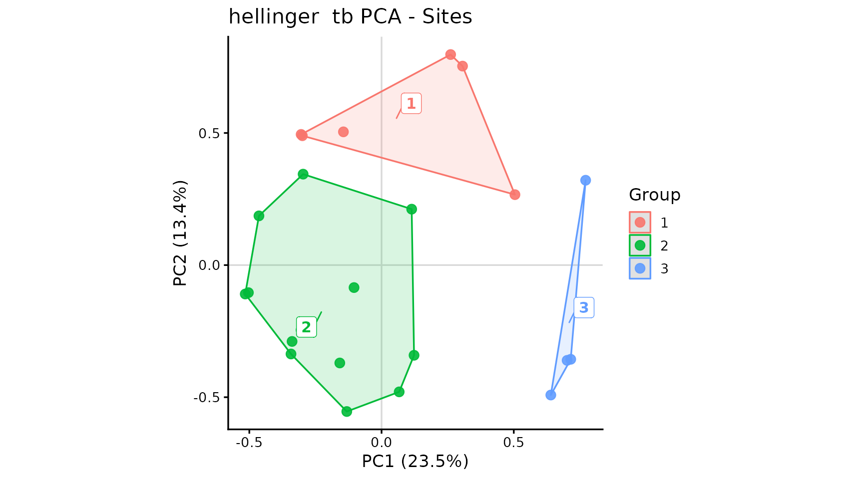

pca$plot_species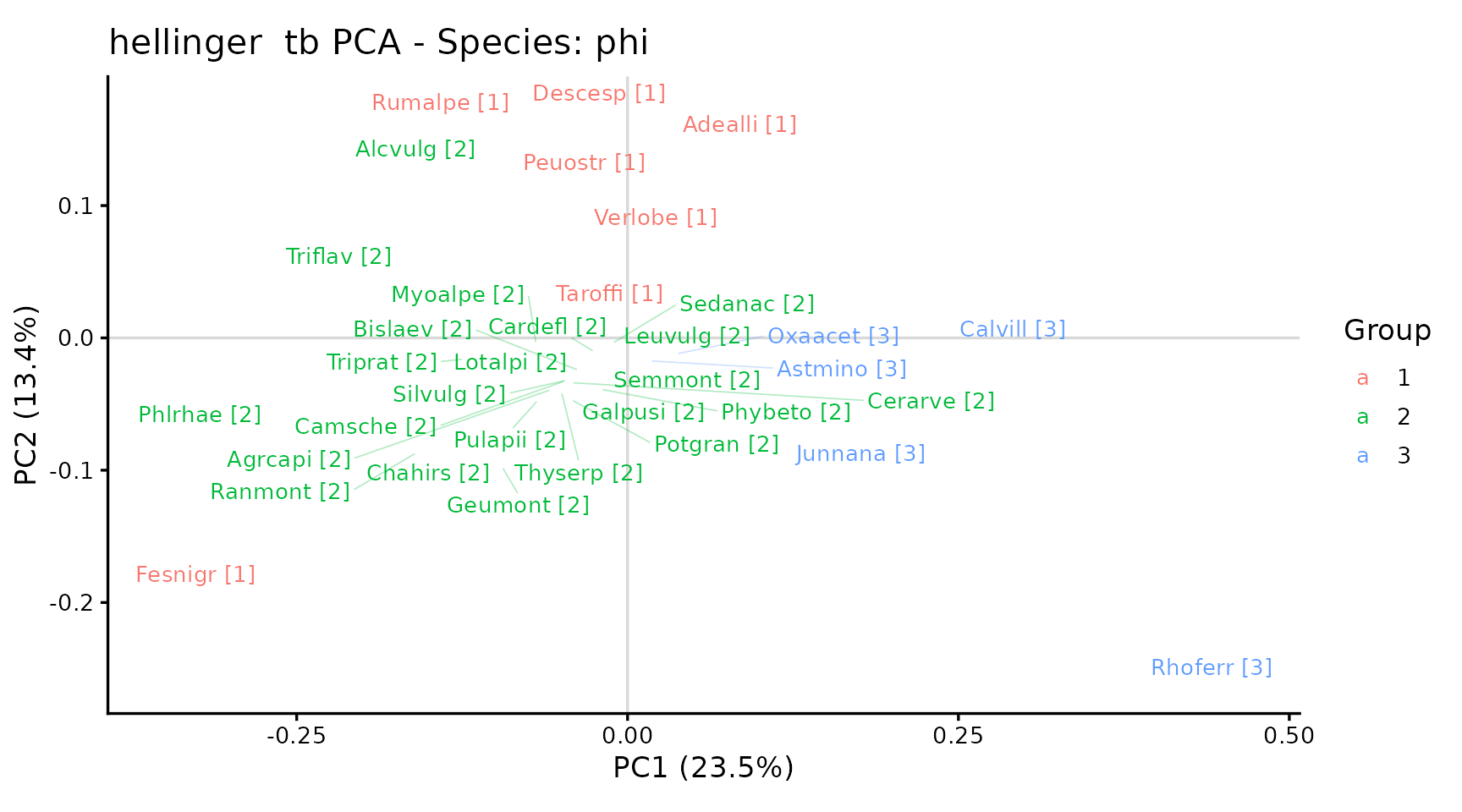

Convex hulls describe the distribution of surveys in the ordination plane and are not confidence intervals. Interpret the plots alongside the variance explained by the axes and the composition of the groups.

pca$variance
#>       PC1       PC2       PC3       PC4       PC5       PC6       PC7       PC8 
#> 23.488587 13.406154  9.954948  8.380961  6.260246  5.039406  4.712287  4.323490 
#>       PC9      PC10      PC11      PC12      PC13      PC14      PC15      PC16 
#>  3.515914  3.068504  2.780572  2.386132  2.187248  1.913238  1.723395  1.681543 
#>      PC17      PC18      PC19      PC20      PC21      PC22      PC23 
#>  1.246019  0.935621  0.771616  0.731182  0.642876  0.484845  0.365215
head(pca$sites)
#>    stand          x           y group
#> R1    R1 -0.1314824 -0.55416009     2
#> R2    R2 -0.1442085  0.50428595     1
#> R3    R3 -0.2994681  0.48959336     1
#> R4    R4 -0.3041198  0.49455601     1
#> R5    R5 -0.5034762 -0.10429268     2
#> R6    R6 -0.1040882 -0.08507569     2
head(pca$species)
#>         species           x           y group
#> Adealli Adealli  0.05351652  0.14810718     1
#> Agrcapi Agrcapi -0.05776389 -0.03908370     2
#> Alcvulg Alcvulg -0.18558879  0.12936321     2
#> Astmino Astmino  0.01702381 -0.01739060     3
#> Bislaev Bislaev -0.03698051 -0.02450444     2
#> Calvill Calvill  0.26594510  0.02080365     3
pca$selected_species
#>  [1] "Adealli" "Agrcapi" "Alcvulg" "Astmino" "Bislaev" "Calvill" "Camsche"
#>  [8] "Cardefl" "Cerarve" "Chahirs" "Descesp" "Fesnigr" "Galpusi" "Geumont"
#> [15] "Junnana" "Leuvulg" "Lotalpi" "Myoalpe" "Oxaacet" "Peuostr" "Phlrhae"
#> [22] "Phybeto" "Potgran" "Pulapii" "Ranmont" "Rhoferr" "Rumalpe" "Sedanac"
#> [29] "Semmont" "Silvulg" "Taroffi" "Thyserp" "Triprat" "Triflav" "Verlobe"

8. Synoptic table

Build the synoptic table from the original cover values and the partition already used for ISA, phi, and PCA. The operational definitions in this example are:

• diagnostic: phi of at least 0.25 and an unadjusted p-value no greater than 0.05;
• constant: present in at least 40% of surveys within the group;
• dominant: cover of at least 25% in at least 50% of surveys within the group.

The last definition corresponds to dominance_rule = "high_cover_frequency". It does not simply mean a mean cover of at least 25% within the group. The three categories may overlap.

stopifnot(
  identical(rownames(phi$sign), colnames(veg)),
  identical(as.character(phi$cluster), as.character(groups$group))
)

tab_sinottica <- synoptic_table(
  veg = veg,
  groups = groups$group,
  phi = phi,
  alpha = 0.05,
  phi_min = 0.25,
  constancy_min = 40,
  dominant_freq_min = 50,
  dominant_cover_min = 25,
  include = c("diagnostic", "constant", "dominant"),
  dominance_rule = "high_cover_frequency"
)

knitr::kable(head(tab_sinottica$synoptic, 20))

group	species	diagnostic	phi	p.value	frequency	constant	high_cover_frequency	max_cover	dominant	G1	G2	G3
1	Rumalpe	TRUE	0.555	0.015	100.0	TRUE	16.7	64.0	FALSE	100.0	85.7	0
1	Fesnigr	TRUE	0.408	0.015	100.0	TRUE	16.7	32.0	FALSE	100.0	100.0	25
1	Peuostr	TRUE	0.553	0.040	83.3	TRUE	16.7	48.0	FALSE	83.3	50.0	0
1	Adealli	TRUE	0.756	0.005	66.7	TRUE	16.7	32.0	FALSE	66.7	0.0	0
1	Verlobe	TRUE	0.691	0.035	66.7	TRUE	0.0	20.0	FALSE	66.7	7.1	0
1	Descesp	TRUE	0.557	0.030	50.0	TRUE	33.3	92.0	FALSE	50.0	7.1	0
1	Taroffi	TRUE	0.557	0.040	50.0	TRUE	0.0	0.3	FALSE	50.0	7.1	0
1	Alcvulg	FALSE	NA	NA	100.0	TRUE	0.0	24.0	FALSE	100.0	100.0	0
1	Agrcapi	FALSE	NA	NA	83.3	TRUE	16.7	28.0	FALSE	83.3	100.0	50
1	Phlrhae	FALSE	NA	NA	83.3	TRUE	33.3	44.0	FALSE	83.3	100.0	0
1	Poaalpi	FALSE	NA	NA	83.3	TRUE	0.0	16.0	FALSE	83.3	71.4	0
1	Antalpi	FALSE	NA	NA	66.7	TRUE	0.0	4.0	FALSE	66.7	85.7	25
1	Chahirs	FALSE	NA	NA	66.7	TRUE	0.0	0.3	FALSE	66.7	92.9	0
1	Luzalpi	FALSE	NA	NA	66.7	TRUE	0.0	4.0	FALSE	66.7	21.4	0
1	Viobifl	FALSE	NA	NA	66.7	TRUE	0.0	20.0	FALSE	66.7	57.1	0
1	Alnviri	FALSE	NA	NA	50.0	TRUE	33.3	92.0	FALSE	50.0	7.1	25
1	Camsche	FALSE	NA	NA	50.0	TRUE	0.0	0.3	FALSE	50.0	92.9	0
1	Cervulg	FALSE	NA	NA	50.0	TRUE	0.0	0.3	FALSE	50.0	21.4	0
1	Gersylv	FALSE	NA	NA	50.0	TRUE	0.0	4.0	FALSE	50.0	57.1	0
1	Ranmont	FALSE	NA	NA	50.0	TRUE	0.0	4.0	FALSE	50.0	92.9	0

With duleg = TRUE, multipatt() returns the single group with the strongest association for each species. The synoptic table uses that selection for diagnostic species; it does not list all possible species-by-group comparisons. A species may nevertheless be constant or dominant in several groups.

The main table is in long format: a species may appear in multiple rows, one for each group in which it meets the requested category criteria. The frequency matrix includes all species and reports their percentage frequencies within groups.

# Diagnostic species only.
diagnostic_species <- subset(tab_sinottica$synoptic, diagnostic)
knitr::kable(head(diagnostic_species, 20))

	group	species	diagnostic	phi	p.value	frequency	constant	high_cover_frequency	max_cover	dominant	G1	G2	G3
1	1	Rumalpe	TRUE	0.555	0.015	100.0	TRUE	16.7	64.0	FALSE	100.0	85.7	0
2	1	Fesnigr	TRUE	0.408	0.015	100.0	TRUE	16.7	32.0	FALSE	100.0	100.0	25
3	1	Peuostr	TRUE	0.553	0.040	83.3	TRUE	16.7	48.0	FALSE	83.3	50.0	0
4	1	Adealli	TRUE	0.756	0.005	66.7	TRUE	16.7	32.0	FALSE	66.7	0.0	0
5	1	Verlobe	TRUE	0.691	0.035	66.7	TRUE	0.0	20.0	FALSE	66.7	7.1	0
6	1	Descesp	TRUE	0.557	0.030	50.0	TRUE	33.3	92.0	FALSE	50.0	7.1	0
7	1	Taroffi	TRUE	0.557	0.040	50.0	TRUE	0.0	0.3	FALSE	50.0	7.1	0
23	2	Phlrhae	TRUE	0.564	0.005	100.0	TRUE	35.7	44.0	FALSE	83.3	100.0	0
24	2	Alcvulg	TRUE	0.500	0.010	100.0	TRUE	7.1	72.0	FALSE	100.0	100.0	0
25	2	Agrcapi	TRUE	0.378	0.020	100.0	TRUE	21.4	60.0	FALSE	83.3	100.0	50
26	2	Myoalpe	TRUE	0.828	0.005	92.9	TRUE	7.1	40.0	FALSE	16.7	92.9	0
27	2	Camsche	TRUE	0.640	0.005	92.9	TRUE	0.0	8.0	FALSE	50.0	92.9	0
28	2	Ranmont	TRUE	0.640	0.005	92.9	TRUE	14.3	36.0	FALSE	50.0	92.9	0
29	2	Chahirs	TRUE	0.562	0.010	92.9	TRUE	7.1	28.0	FALSE	66.7	92.9	0
30	2	Phybeto	TRUE	0.715	0.005	85.7	TRUE	0.0	4.0	FALSE	0.0	85.7	25
31	2	Geumont	TRUE	0.665	0.005	85.7	TRUE	0.0	24.0	FALSE	33.3	85.7	0
32	2	Lotalpi	TRUE	0.665	0.005	85.7	TRUE	0.0	4.0	FALSE	33.3	85.7	0
33	2	Triprat	TRUE	0.665	0.005	85.7	TRUE	0.0	24.0	FALSE	33.3	85.7	0
34	2	Cerarve	TRUE	0.842	0.005	78.6	TRUE	0.0	8.0	FALSE	0.0	78.6	0
35	2	Silvulg	TRUE	0.603	0.015	78.6	TRUE	7.1	28.0	FALSE	33.3	78.6	0

# Diagnostic or constant species in group 2.
group2_species <- subset(
  tab_sinottica$synoptic,
  (diagnostic | constant) & as.character(group) == "2"
)
knitr::kable(head(group2_species, 20))

	group	species	diagnostic	phi	p.value	frequency	constant	high_cover_frequency	max_cover	dominant	G1	G2	G3
23	2	Phlrhae	TRUE	0.564	0.005	100.0	TRUE	35.7	44	FALSE	83.3	100.0	0
24	2	Alcvulg	TRUE	0.500	0.010	100.0	TRUE	7.1	72	FALSE	100.0	100.0	0
25	2	Agrcapi	TRUE	0.378	0.020	100.0	TRUE	21.4	60	FALSE	83.3	100.0	50
26	2	Myoalpe	TRUE	0.828	0.005	92.9	TRUE	7.1	40	FALSE	16.7	92.9	0
27	2	Camsche	TRUE	0.640	0.005	92.9	TRUE	0.0	8	FALSE	50.0	92.9	0
28	2	Ranmont	TRUE	0.640	0.005	92.9	TRUE	14.3	36	FALSE	50.0	92.9	0
29	2	Chahirs	TRUE	0.562	0.010	92.9	TRUE	7.1	28	FALSE	66.7	92.9	0
30	2	Phybeto	TRUE	0.715	0.005	85.7	TRUE	0.0	4	FALSE	0.0	85.7	25
31	2	Geumont	TRUE	0.665	0.005	85.7	TRUE	0.0	24	FALSE	33.3	85.7	0
32	2	Lotalpi	TRUE	0.665	0.005	85.7	TRUE	0.0	4	FALSE	33.3	85.7	0
33	2	Triprat	TRUE	0.665	0.005	85.7	TRUE	0.0	24	FALSE	33.3	85.7	0
34	2	Cerarve	TRUE	0.842	0.005	78.6	TRUE	0.0	8	FALSE	0.0	78.6	0
35	2	Silvulg	TRUE	0.603	0.015	78.6	TRUE	7.1	28	FALSE	33.3	78.6	0
36	2	Potgran	TRUE	0.791	0.010	71.4	TRUE	0.0	8	FALSE	0.0	71.4	0
37	2	Triflav	TRUE	0.653	0.005	71.4	TRUE	28.6	36	FALSE	16.7	71.4	0
38	2	Galpusi	TRUE	0.739	0.025	64.3	TRUE	0.0	8	FALSE	0.0	64.3	0
39	2	Pulapii	TRUE	0.739	0.010	64.3	TRUE	0.0	24	FALSE	0.0	64.3	0
40	2	Cardefl	TRUE	0.534	0.045	57.1	TRUE	0.0	8	FALSE	16.7	57.1	0
41	2	Sedanac	TRUE	0.534	0.045	57.1	TRUE	0.0	4	FALSE	16.7	57.1	0
42	2	Bislaev	TRUE	0.632	0.020	50.0	TRUE	0.0	12	FALSE	0.0	50.0	0

# Percentage frequencies of all species.
head(tab_sinottica$frequency)
#>               G1        G2 G3
#> Achmacr 33.33333  0.000000  0
#> Achmill  0.00000 42.857143  0
#> Achmosc  0.00000 14.285714  0
#> Acialpi  0.00000 28.571429  0
#> Acolama 33.33333  7.142857  0
#> Adealli 66.66667  0.000000  0

# Diagnostic species and their associations.
head(tab_sinottica$diagnostic)
#>   species diagnostic diagnostic_group       phi p.value
#> 1 Adealli       TRUE                1 0.7559289   0.005
#> 2 Agrcapi       TRUE                2 0.3779645   0.020
#> 3 Alcvulg       TRUE                2 0.5000000   0.010
#> 4 Astmino       TRUE                3 0.5442535   0.045
#> 5 Bislaev       TRUE                2 0.6324555   0.020
#> 6 Calvill       TRUE                3 0.6328612   0.030

9. Optional export

The first chunk saves results and frequencies using base R functions. Both export chunks are excluded from normal rendering.

output_dir <- "risultati_fitosociologia"
dir.create(output_dir, recursive = TRUE, showWarnings = FALSE)

write.csv2(groups, file.path(output_dir, "gruppi.csv"), row.names = FALSE)
write.csv2(
  group_key,
  file.path(output_dir, "corrispondenza_gruppi.csv"),
  row.names = FALSE
)
write.csv2(
  twinspan_res$results,
  file.path(output_dir, "optimclass.csv"),
  row.names = FALSE
)
write.csv2(indval_table, file.path(output_dir, "indval.csv"), row.names = FALSE)
write.csv2(phi_table, file.path(output_dir, "phi.csv"), row.names = FALSE)
write.csv2(
  tab_sinottica$synoptic,
  file.path(output_dir, "sinottica_lunga.csv"),
  row.names = FALSE
)

frequency_table <- data.frame(
  species = rownames(tab_sinottica$frequency),
  tab_sinottica$frequency,
  row.names = NULL,
  check.names = FALSE
)
write.csv2(
  frequency_table,
  file.path(output_dir, "frequenze.csv"),
  row.names = FALSE
)

saveRDS(
  list(
    veg = veg,
    optimclass = twinspan_res,
    n.cluster = n.cluster,
    groups = groups,
    group_key = group_key,
    indval = indval,
    phi = phi,
    pca = pca,
    synoptic = tab_sinottica,
    permutations = permutation_matrix,
    parameters = list(
      cut_levels = cut_levels,
      min_size = min_size,
      k_values = k_values,
      p_threshold = p_threshold,
      min_faithful = min_faithful,
      select_by = select_by,
      occasional_cover = occasional_cover
    ),
    session = sessionInfo()
  ),
  file.path(output_dir, "analisi_fitosociologica.rds")
)

If export_synoptic() is also available, export an abbreviated synoptic table to Excel. In the interface used here, min_frequency = 30 retains all diagnostic species and, among the other species in the input synoptic table, those with a frequency of at least 30% in one group. It does not restore species already excluded by include when building the table.

stopifnot(exists("export_synoptic", mode = "function"))

export_synoptic(
  tab_sinottica$synoptic,
  file = "Sinottica_short.xlsx",
  min_frequency = 30,
  digits = 1,
  group_sizes = table(groups$group)
)

Function references

• iPastoralist documentation and source code.
• TWINSPAN in the ecan package.
• OptimClass: Tichý et al. (2010).
• multipatt documentation.